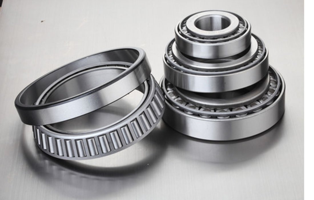
In the world of mechanical engineering, bearings are often hailed as the “joints of machinery.” From the traction motors driving high-speed trains to the precise joints of industrial robots, bearings quietly endure high speeds and heavy loads behind the scenes. However, no bearing can rotate indefinitely.

In bearing design and selection, there is one critical parameter that takes center stage: Basic Rating Life. It is not only the yardstick for measuring bearing durability but also the golden rule for balancing safety and cost-effectiveness in engineering design.

1. What is Bearing Rating Life?

When we talk about the “life” of a bearing, what exactly do we mean? Is it the exact moment the bearing completely seizes, or is it when it first starts making an unusual noise?

In academic and industrial standards (such as ISO 281), the rating life of a bearing has a strict definition. It is commonly referred to as the $L_{10}$ life:

$L_{10}$ Basic Rating Life: The life associated with a 90% reliability for a group of apparently identical bearings operating under identical conditions. It represents the number of revolutions (in millions of revolutions, $10^6$) or operating hours at a given speed that 90% of the bearings will achieve or exceed before the first evidence of fatigue spalling or pitting develops.

In other words, if 100 identical bearings run under the exact same operating conditions, by the time they reach their $L_{10}$ life, a maximum of 10 bearings will have failed due to metal fatigue, while the remaining 90 will still be fully functional.

2. The Mathematical Beauty of Longevity: The Fatigue Life Formula

The rating life of a bearing is not a guess; it is derived from empirical formulas based on the classic Lundberg-Palmgren theory:

Where each parameter holds a specific physical significance:

• $L_{10}$: Basic rating life (in millions of revolutions, $10^6$).

• $C$ (Basic Dynamic Load Rating)：The constant radial (or axial) load that a bearing can theoretically endure for one million revolutions without experiencing fatigue failure.

• $P$ (Equivalent Dynamic Load)：Since real-world bearings often bear a combination of radial and axial forces, the actual composite force must be converted into a single equivalent dynamic load using standard formulas.

• $p$ (Life Exponent)：This depends on the geometry of the rolling elements.

  • For ball bearings (point contact), $p = 3$.

  • For roller bearings (line contact), $p = 10/3 \approx 3.33$.

The Power of the Exponent

As shown in the formula, life is inversely proportional to the load ratio ($C/P$) raised to the third or higher power. This means that if the actual load $P$ is doubled, the life of a ball bearing will plummet to just $\frac{1}{2^3} = \frac{1}{8}$ of its original value! Conversely, even a minor reduction in load can trigger an exponential increase in bearing lifespan.

3. Why Do Identical Bearings Have Vastly Different Lifespans?

In practical engineering, designers are often puzzled: “Why is it that out of two identical bearings bought from the same batch and installed on the same machine, one lasts five years while the other fails in six months?”

This highlights the unique characteristic of bearing life: extreme statistical dispersion.

Macro-Fatigue and Micro-Randomness

The primary cause of bearing failure is rolling contact fatigue. As rolling elements repeatedly pass over the raceways, intense alternating stresses accumulate beneath the metal surface. Because steel naturally contains microscopic non-metallic inclusions, tiny voids, or crystal defects, the exact point where a micro-crack initiates and propagates to the surface is highly random.

The Weibull Distribution

Statistical analysis shows that bearing life follows the Weibull Distribution. Within the exact same batch, the longest-living bearing might last dozens or even hundreds of times longer than the shortest-living one. Consequently, predicting the exact “death date” of a single, specific bearing is virtually impossible. This is why engineering must rely on the $L_{10}$ concept to guarantee system reliability through probability.

4. Moving into Reality: Modified Rating Life ($L_{nm}$)

With rapid advancements in material science and lubrication technology, the traditional $L_{10}$ formula can sometimes be overly conservative. If a bearing operates under ideal conditions—extreme cleanliness, optimal lubrication, and light loads—it can theoretically achieve an infinite lifespan.

To account for this, modern ISO standards introduce the Modified Rating Life formula:

• $a_1$ (Reliability Factor)：If high-stakes industries like aerospace demand a 99% or 99.9% reliability rate (i.e., $L_1$ or $L_{0.1}$ life), this factor drops below 1 to compress the calculated safe lifespan.

• $a_{ISO}$ (System Modification Factor)：A highly sophisticated factor that evaluates lubricant viscosity, operating temperature, oil film thickness ratio ($\kappa$), and particulate contamination. In clean, perfectly lubricated environments, this factor can be significantly greater than 1, drastically extending the calculated life.

5. The Art of Balance in Bearing Design

In mechanical design, a longer rating life is not always better. Blindly pursuing an excessively long lifespan leads to oversized bearings. This not only adds unnecessary weight and bulk to the machine (increasing rotational inertia) but also drives up manufacturing costs.

Experienced engineers always align their target rating life with the specific application scenario:

• Short-term or Intermittent Operations (e.g., household power tools, automotive window lifters): A design life of just a few hundred to a few thousand hours is often sufficient.

• Continuous, High-Reliability Operations (e.g., power plant generators, paper-making machinery, large marine propulsion systems): The design life typically demands 50,000 to over 100,000 hours.

Conclusion

The rating life of a bearing serves as a bridge between cold, rigid mechanical equations and the chaotic randomness of physical reality. It reminds designers that engineering is not about chasing absolute eternity, but about finding the optimal equilibrium between probability and cost. Mastering the essence of rating life allows us to do more than just pick the right part—it empowers us to navigate complex mechanical systems with profound respect for physical laws and absolute confidence in design.